Vectors and Parallel Data

The vector (denoted by Vec) is one of the simplest PETSc objects. Vectors are used to store discrete PDE solutions, right-hand sides for linear systems, etc. This chapter is organized as follows:

• (Vec) Creating and Assembling Vectors and Basic Vector Operations - basic usage of vectors

• Section Indexing and Ordering - management of the various numberings of degrees of freedom, vertices, cells, etc.

  • (AO) Mapping between different global numberings

  • (ISLocalToGlobalMapping) Mapping between local and global numberings

• (DM) Structured Grids Using Distributed Arrays - management of grids

• (IS, VecScatter) Vectors Related to Unstructured Grids - management of vectors related to unstructured grids

Creating and Assembling Vectors

PETSc currently provides two basic vector types: sequential and parallel (MPI-based). To create a sequential vector with m components, one can use the command

VecCreateSeq(PETSC_COMM_SELF,PetscInt m,Vec *x);

To create a parallel vector one can either specify the number of components that will be stored on each process or let PETSc decide. The command

VecCreateMPI(MPI_Comm comm,PetscInt m,PetscInt M,Vec *x);

creates a vector distributed over all processes in the communicator, comm, where m indicates the number of components to store on the local process, and M is the total number of vector components. Either the local or global dimension, but not both, can be set to PETSC_DECIDE or PETSC_DETERMINE, respectively, to indicate that PETSc should decide or determine it. More generally, one can use the routines

VecCreate(MPI_Comm comm,Vec *v);
VecSetSizes(Vec v, PetscInt m, PetscInt M);
VecSetFromOptions(Vec v);

which automatically generates the appropriate vector type (sequential or parallel) over all processes in comm. The option -vec_type mpi can be used in conjunction with VecCreate() and VecSetFromOptions() to specify the use of MPI vectors even for the uniprocessor case.

We emphasize that all processes in comm must call the vector creation routines, since these routines are collective over all processes in the communicator. If you are not familiar with MPI communicators, see the discussion in Writing PETSc Programs on page . In addition, if a sequence of VecCreateXXX() routines is used, they must be called in the same order on each process in the communicator.

One can assign a single value to all components of a vector with the command

VecSet(Vec x,PetscScalar value);

Assigning values to individual components of the vector is more complicated, in order to make it possible to write efficient parallel code. Assigning a set of components is a two-step process: one first calls

VecSetValues(Vec x,PetscInt n,PetscInt *indices,PetscScalar *values,INSERT_VALUES);

any number of times on any or all of the processes. The argument n gives the number of components being set in this insertion. The integer array indices contains the global component indices, and values is the array of values to be inserted. Any process can set any components of the vector; PETSc ensures that they are automatically stored in the correct location. Once all of the values have been inserted with VecSetValues(), one must call

VecAssemblyBegin(Vec x);

followed by

VecAssemblyEnd(Vec x);

to perform any needed message passing of nonlocal components. In order to allow the overlap of communication and calculation, the user’s code can perform any series of other actions between these two calls while the messages are in transition.

Example usage of VecSetValues() may be found in $PETSC_DIR/src/vec/vec/tutorials/ex2.c or ex2f.F.

Often, rather than inserting elements in a vector, one may wish to add values. This process is also done with the command

VecSetValues(Vec x,PetscInt n,PetscInt *indices, PetscScalar *values,ADD_VALUES);

Again one must call the assembly routines VecAssemblyBegin() and VecAssemblyEnd() after all of the values have been added. Note that addition and insertion calls to VecSetValues() cannot be mixed. Instead, one must add and insert vector elements in phases, with intervening calls to the assembly routines. This phased assembly procedure overcomes the nondeterministic behavior that would occur if two different processes generated values for the same location, with one process adding while the other is inserting its value. (In this case the addition and insertion actions could be performed in either order, thus resulting in different values at the particular location. Since PETSc does not allow the simultaneous use of INSERT_VALUES and ADD_VALUES this nondeterministic behavior will not occur in PETSc.)

You can call VecGetValues() to pull local values from a vector (but not off-process values), an alternative method for extracting some components of a vector are the vector scatter routines. See Scatters and Gathers for details; see also below for VecGetArray().

One can examine a vector with the command

VecView(Vec x,PetscViewer v);

To print the vector to the screen, one can use the viewer PETSC_VIEWER_STDOUT_WORLD, which ensures that parallel vectors are printed correctly to stdout. To display the vector in an X-window, one can use the default X-windows viewer PETSC_VIEWER_DRAW_WORLD, or one can create a viewer with the routine PetscViewerDrawOpenX(). A variety of viewers are discussed further in Viewers: Looking at PETSc Objects.

To create a new vector of the same format as an existing vector, one uses the command

VecDuplicate(Vec old,Vec *new);

To create several new vectors of the same format as an existing vector, one uses the command

VecDuplicateVecs(Vec old,PetscInt n,Vec **new);

This routine creates an array of pointers to vectors. The two routines are very useful because they allow one to write library code that does not depend on the particular format of the vectors being used. Instead, the subroutines can automatically correctly create work vectors based on the specified existing vector. As discussed in Duplicating Multiple Vectors, the Fortran interface for VecDuplicateVecs() differs slightly.

When a vector is no longer needed, it should be destroyed with the command

VecDestroy(Vec *x);

To destroy an array of vectors, use the command

VecDestroyVecs(PetscInt n,Vec **vecs);

Note that the Fortran interface for VecDestroyVecs() differs slightly, as described in Duplicating Multiple Vectors.

It is also possible to create vectors that use an array provided by the user, rather than having PETSc internally allocate the array space. Such vectors can be created with the routines

VecCreateSeqWithArray(PETSC_COMM_SELF,PetscInt bs,PetscInt n,PetscScalar *array,Vec *V);

and

VecCreateMPIWithArray(MPI_Comm comm,PetscInt bs,PetscInt n,PetscInt N,PetscScalar *array,Vec *vv);

Note that here one must provide the value n; it cannot be PETSC_DECIDE and the user is responsible for providing enough space in the array; n*sizeof(PetscScalar).

Basic Vector Operations

Table 1 PETSc Vector Operations

Function Name	Operation
VecAXPY(Vec y,PetscScalar a,Vec x);	\(y = y + a*x\)
VecAYPX(Vec y,PetscScalar a,Vec x);	\(y = x + a*y\)
VecWAXPY(Vec  w,PetscScalar a,Vec x,Vec y);	\(w = a*x + y\)
VecAXPBY(Vec y,PetscScalar a,PetscScalar b,Vec x);	\(y = a*x + b*y\)
VecScale(Vec x, PetscScalar a);	\(x = a*x\)
VecDot(Vec x, Vec y, PetscScalar *r);	\(r = \bar{x}^T*y\)
VecTDot( Vec x, Vec y, PetscScalar *r);	\(r = x'*y\)
VecNorm(Vec x, NormType type,  PetscReal *r);	\(r = ||x||_{type}\)
VecSum(Vec x, PetscScalar *r);	\(r = \sum x_{i}\)
VecCopy(Vec x, Vec y);	\(y = x\)
VecSwap(Vec x, Vec y);	\(y = x\) while \(x = y\)
VecPointwiseMult(Vec w,Vec x,Vec y);	\(w_{i} = x_{i}*y_{i}\)
VecPointwiseDivide(Vec w,Vec x,Vec y);	\(w_{i} = x_{i}/y_{i}\)
VecMDot(Vec x,PetscInt n,Vec y[],PetscScalar *r);	\(r[i] = \bar{x}^T*y[i]\)
VecMTDot(Vec x,PetscInt n,Vec y[],PetscScalar *r);	\(r[i] = x^T*y[i]\)
VecMAXPY(Vec y,PetscInt n, PetscScalar *a, Vec x[]);	\(y = y + \sum_i a_{i}*x[i]\)
VecMax(Vec x, PetscInt *idx, PetscReal *r);	\(r = \max x_{i}\)
VecMin(Vec x, PetscInt *idx, PetscReal *r);	\(r = \min x_{i}\)
VecAbs(Vec x);	\(x_i = |x_{i}|\)
VecReciprocal(Vec x);	\(x_i = 1/x_{i}\)
VecShift(Vec x,PetscScalar s);	\(x_i = s + x_{i}\)
VecSet(Vec x,PetscScalar alpha);	\(x_i = \alpha\)

As listed in the table, we have chosen certain basic vector operations to support within the PETSc vector library. These operations were selected because they often arise in application codes. The NormType argument to VecNorm() is one of NORM_1, NORM_2, or NORM_INFINITY. The 1-norm is \(\sum_i |x_{i}|\), the 2-norm is \(( \sum_{i} x_{i}^{2})^{1/2}\) and the infinity norm is \(\max_{i} |x_{i}|\).

For parallel vectors that are distributed across the processes by ranges, it is possible to determine a process’s local range with the routine

VecGetOwnershipRange(Vec vec,PetscInt *low,PetscInt *high);

The argument low indicates the first component owned by the local process, while high specifies one more than the last owned by the local process. This command is useful, for instance, in assembling parallel vectors.

On occasion, the user needs to access the actual elements of the vector. The routine VecGetArray() returns a pointer to the elements local to the process:

VecGetArray(Vec v,PetscScalar **array);

When access to the array is no longer needed, the user should call

VecRestoreArray(Vec v, PetscScalar **array);

If the values do not need to be modified, the routines VecGetArrayRead() and VecRestoreArrayRead() provide read-only access and should be used instead.

VecGetArrayRead(Vec v, const PetscScalar **array);
VecRestoreArrayRead(Vec v, const PetscScalar **array);

Minor differences exist in the Fortran interface for VecGetArray() and VecRestoreArray(), as discussed in Array Arguments. It is important to note that VecGetArray() and VecRestoreArray() do not copy the vector elements; they merely give users direct access to the vector elements. Thus, these routines require essentially no time to call and can be used efficiently.

The number of elements stored locally can be accessed with

VecGetLocalSize(Vec v,PetscInt *size);

The global vector length can be determined by

VecGetSize(Vec v,PetscInt *size);

In addition to VecDot() and VecMDot() and VecNorm(), PETSc provides split phase versions of these that allow several independent inner products and/or norms to share the same communication (thus improving parallel efficiency). For example, one may have code such as

VecDot(Vec x,Vec y,PetscScalar *dot);
VecMDot(Vec x,PetscInt nv, Vec y[],PetscScalar *dot);
VecNorm(Vec x,NormType NORM_2,PetscReal *norm2);
VecNorm(Vec x,NormType NORM_1,PetscReal *norm1);

This code works fine, but it performs three separate parallel communication operations. Instead, one can write

VecDotBegin(Vec x,Vec y,PetscScalar *dot);
VecMDotBegin(Vec x, PetscInt nv,Vec y[],PetscScalar *dot);
VecNormBegin(Vec x,NormType NORM_2,PetscReal *norm2);
VecNormBegin(Vec x,NormType NORM_1,PetscReal *norm1);
VecDotEnd(Vec x,Vec y,PetscScalar *dot);
VecMDotEnd(Vec x, PetscInt nv,Vec y[],PetscScalar *dot);
VecNormEnd(Vec x,NormType NORM_2,PetscReal *norm2);
VecNormEnd(Vec x,NormType NORM_1,PetscReal *norm1);

With this code, the communication is delayed until the first call to VecxxxEnd() at which a single MPI reduction is used to communicate all the required values. It is required that the calls to the VecxxxEnd() are performed in the same order as the calls to the VecxxxBegin(); however, if you mistakenly make the calls in the wrong order, PETSc will generate an error informing you of this. There are additional routines VecTDotBegin() and VecTDotEnd(), VecMTDotBegin(), VecMTDotEnd().

Note: these routines use only MPI-1 functionality; they do not allow you to overlap computation and communication (assuming no threads are spawned within a MPI process). Once MPI-2 implementations are more common we’ll improve these routines to allow overlap of inner product and norm calculations with other calculations. Also currently these routines only work for the PETSc built in vector types.

Indexing and Ordering

When writing parallel PDE codes, there is extra complexity caused by having multiple ways of indexing (numbering) and ordering objects such as vertices and degrees of freedom. For example, a grid generator or partitioner may renumber the nodes, requiring adjustment of the other data structures that refer to these objects; see Figure Natural Ordering and PETSc Ordering for a 2D Distributed Array (Four Processes). In addition, local numbering (on a single process) of objects may be different than the global (cross-process) numbering. PETSc provides a variety of tools to help to manage the mapping amongst the various numbering systems. The two most basic are the AO (application ordering), which enables mapping between different global (cross-process) numbering schemes and the ISLocalToGlobalMapping, which allows mapping between local (on-process) and global (cross-process) numbering.

Application Orderings

In many applications it is desirable to work with one or more “orderings” (or numberings) of degrees of freedom, cells, nodes, etc. Doing so in a parallel environment is complicated by the fact that each process cannot keep complete lists of the mappings between different orderings. In addition, the orderings used in the PETSc linear algebra routines (often contiguous ranges) may not correspond to the “natural” orderings for the application.

PETSc provides certain utility routines that allow one to deal cleanly and efficiently with the various orderings. To define a new application ordering (called an AO in PETSc), one can call the routine

AOCreateBasic(MPI_Comm comm,PetscInt n,const PetscInt apordering[],const PetscInt petscordering[],AO *ao);

The arrays apordering and petscordering, respectively, contain a list of integers in the application ordering and their corresponding mapped values in the PETSc ordering. Each process can provide whatever subset of the ordering it chooses, but multiple processes should never contribute duplicate values. The argument n indicates the number of local contributed values.

For example, consider a vector of length 5, where node 0 in the application ordering corresponds to node 3 in the PETSc ordering. In addition, nodes 1, 2, 3, and 4 of the application ordering correspond, respectively, to nodes 2, 1, 4, and 0 of the PETSc ordering. We can write this correspondence as

\[\{ 0, 1, 2, 3, 4 \} \to \{ 3, 2, 1, 4, 0 \}. \]

The user can create the PETSc AO mappings in a number of ways. For example, if using two processes, one could call

AOCreateBasic(PETSC_COMM_WORLD,2,{0,3},{3,4},&ao);

on the first process and

AOCreateBasic(PETSC_COMM_WORLD,3,{1,2,4},{2,1,0},&ao);

on the other process.

Once the application ordering has been created, it can be used with either of the commands

AOPetscToApplication(AO ao,PetscInt n,PetscInt *indices);
AOApplicationToPetsc(AO ao,PetscInt n,PetscInt *indices);

Upon input, the n-dimensional array indices specifies the indices to be mapped, while upon output, indices contains the mapped values. Since we, in general, employ a parallel database for the AO mappings, it is crucial that all processes that called AOCreateBasic() also call these routines; these routines cannot be called by just a subset of processes in the MPI communicator that was used in the call to AOCreateBasic().

An alternative routine to create the application ordering, AO, is

AOCreateBasicIS(IS apordering,IS petscordering,AO *ao);

where index sets (see Index Sets) are used instead of integer arrays.

The mapping routines

AOPetscToApplicationIS(AO ao,IS indices);
AOApplicationToPetscIS(AO ao,IS indices);

will map index sets (IS objects) between orderings. Both the AOXxxToYyy() and AOXxxToYyyIS() routines can be used regardless of whether the AO was created with a AOCreateBasic() or AOCreateBasicIS().

The AO context should be destroyed with AODestroy(AO *ao) and viewed with AOView(AO ao,PetscViewer viewer).

Although we refer to the two orderings as “PETSc” and “application” orderings, the user is free to use them both for application orderings and to maintain relationships among a variety of orderings by employing several AO contexts.

The AOxxToxx() routines allow negative entries in the input integer array. These entries are not mapped; they simply remain unchanged. This functionality enables, for example, mapping neighbor lists that use negative numbers to indicate nonexistent neighbors due to boundary conditions, etc.

Local to Global Mappings

In many applications one works with a global representation of a vector (usually on a vector obtained with VecCreateMPI()) and a local representation of the same vector that includes ghost points required for local computation. PETSc provides routines to help map indices from a local numbering scheme to the PETSc global numbering scheme. This is done via the following routines

ISLocalToGlobalMappingCreate(MPI_Comm comm,PetscInt bs,PetscInt N,PetscInt* globalnum,PetscCopyMode mode,ISLocalToGlobalMapping* ctx);
ISLocalToGlobalMappingApply(ISLocalToGlobalMapping ctx,PetscInt n,PetscInt *in,PetscInt *out);
ISLocalToGlobalMappingApplyIS(ISLocalToGlobalMapping ctx,IS isin,IS* isout);
ISLocalToGlobalMappingDestroy(ISLocalToGlobalMapping *ctx);

Here N denotes the number of local indices, globalnum contains the global number of each local number, and ISLocalToGlobalMapping is the resulting PETSc object that contains the information needed to apply the mapping with either ISLocalToGlobalMappingApply() or ISLocalToGlobalMappingApplyIS().

Note that the ISLocalToGlobalMapping routines serve a different purpose than the AO routines. In the former case they provide a mapping from a local numbering scheme (including ghost points) to a global numbering scheme, while in the latter they provide a mapping between two global numbering schemes. In fact, many applications may use both AO and ISLocalToGlobalMapping routines. The AO routines are first used to map from an application global ordering (that has no relationship to parallel processing etc.) to the PETSc ordering scheme (where each process has a contiguous set of indices in the numbering). Then in order to perform function or Jacobian evaluations locally on each process, one works with a local numbering scheme that includes ghost points. The mapping from this local numbering scheme back to the global PETSc numbering can be handled with the ISLocalToGlobalMapping routines.

If one is given a list of block indices in a global numbering, the routine

ISGlobalToLocalMappingApplyBlock(ISLocalToGlobalMapping ctx,ISGlobalToLocalMappingMode type,PetscInt nin,PetscInt idxin[],PetscInt *nout,PetscInt idxout[]);

will provide a new list of indices in the local numbering. Again, negative values in idxin are left unmapped. But, in addition, if type is set to IS_GTOLM_MASK , then nout is set to nin and all global values in idxin that are not represented in the local to global mapping are replaced by -1. When type is set to IS_GTOLM_DROP, the values in idxin that are not represented locally in the mapping are not included in idxout, so that potentially nout is smaller than nin. One must pass in an array long enough to hold all the indices. One can call ISGlobalToLocalMappingApplyBlock() with idxout equal to NULL to determine the required length (returned in nout) and then allocate the required space and call ISGlobalToLocalMappingApplyBlock() a second time to set the values.

Often it is convenient to set elements into a vector using the local node numbering rather than the global node numbering (e.g., each process may maintain its own sublist of vertices and elements and number them locally). To set values into a vector with the local numbering, one must first call

VecSetLocalToGlobalMapping(Vec v,ISLocalToGlobalMapping ctx);

and then call

VecSetValuesLocal(Vec x,PetscInt n,const PetscInt indices[],const PetscScalar values[],INSERT_VALUES);

Now the indices use the local numbering, rather than the global, meaning the entries lie in \([0,n)\) where \(n\) is the local size of the vector.

Structured Grids Using Distributed Arrays

Distributed arrays (DMDAs), which are used in conjunction with PETSc vectors, are intended for use with logically regular rectangular grids when communication of nonlocal data is needed before certain local computations can occur. PETSc distributed arrays are designed only for the case in which data can be thought of as being stored in a standard multidimensional array; thus, DMDAs are not intended for parallelizing unstructured grid problems, etc. DAs are intended for communicating vector (field) information; they are not intended for storing matrices.

For example, a typical situation one encounters in solving PDEs in parallel is that, to evaluate a local function, f(x), each process requires its local portion of the vector x as well as its ghost points (the bordering portions of the vector that are owned by neighboring processes). Figure Ghost Points for Two Stencil Types on the Seventh Process illustrates the ghost points for the seventh process of a two-dimensional, regular parallel grid. Each box represents a process; the ghost points for the seventh process’s local part of a parallel array are shown in gray.

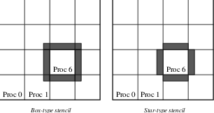
Fig. 2 Ghost Points for Two Stencil Types on the Seventh Process

Creating Distributed Arrays

The PETSc DMDA object manages the parallel communication required while working with data stored in regular arrays. The actual data is stored in appropriately sized vector objects; the DMDA object only contains the parallel data layout information and communication information, however it may be used to create vectors and matrices with the proper layout.

One creates a distributed array communication data structure in two dimensions with the command

DMDACreate2d(MPI_Comm comm,DMBoundaryType xperiod,DMBoundaryType yperiod,DMDAStencilType st,PetscInt M, PetscInt N,PetscInt m,PetscInt n,PetscInt dof,PetscInt s,PetscInt *lx,PetscInt *ly,DM *da);

The arguments M and N indicate the global numbers of grid points in each direction, while m and n denote the process partition in each direction; m*n must equal the number of processes in the MPI communicator, comm. Instead of specifying the process layout, one may use PETSC_DECIDE for m and n so that PETSc will determine the partition using MPI. The type of periodicity of the array is specified by xperiod and yperiod, which can be DM_BOUNDARY_NONE (no periodicity), DM_BOUNDARY_PERIODIC (periodic in that direction), DM_BOUNDARY_TWIST (periodic in that direction, but identified in reverse order), DM_BOUNDARY_GHOSTED , or DM_BOUNDARY_MIRROR. The argument dof indicates the number of degrees of freedom at each array point, and s is the stencil width (i.e., the width of the ghost point region). The optional arrays lx and ly may contain the number of nodes along the x and y axis for each cell, i.e. the dimension of lx is m and the dimension of ly is n; alternately, NULL may be passed in.

Two types of distributed array communication data structures can be created, as specified by st. Star-type stencils that radiate outward only in the coordinate directions are indicated by DMDA_STENCIL_STAR, while box-type stencils are specified by DMDA_STENCIL_BOX. For example, for the two-dimensional case, DMDA_STENCIL_STAR with width 1 corresponds to the standard 5-point stencil, while DMDA_STENCIL_BOX with width 1 denotes the standard 9-point stencil. In both instances the ghost points are identical, the only difference being that with star-type stencils certain ghost points are ignored, decreasing substantially the number of messages sent. Note that the DMDA_STENCIL_STAR stencils can save interprocess communication in two and three dimensions.

These DMDA stencils have nothing directly to do with any finite difference stencils one might chose to use for a discretization; they only ensure that the correct values are in place for application of a user-defined finite difference stencil (or any other discretization technique).

The commands for creating distributed array communication data structures in one and three dimensions are analogous:

DMDACreate1d(MPI_Comm comm,DMBoundaryType xperiod,PetscInt M,PetscInt w,PetscInt s,PetscInt *lc,DM *inra);
DMDACreate3d(MPI_Comm comm,DMBoundaryType xperiod,DMBoundaryType yperiod,DMBoundaryType zperiod, DMDAStencilType stencil_type,PetscInt M,PetscInt N,PetscInt P,PetscInt m,PetscInt n,PetscInt p,PetscInt w,PetscInt s,PetscInt *lx,PetscInt *ly,PetscInt *lz,DM *inra);

The routines to create distributed arrays are collective, so that all processes in the communicator comm must call DACreateXXX().

Local/Global Vectors and Scatters

Each DMDA object defines the layout of two vectors: a distributed global vector and a local vector that includes room for the appropriate ghost points. The DMDA object provides information about the size and layout of these vectors, but does not internally allocate any associated storage space for field values. Instead, the user can create vector objects that use the DMDA layout information with the routines

DMCreateGlobalVector(DM da,Vec *g);
DMCreateLocalVector(DM da,Vec *l);

These vectors will generally serve as the building blocks for local and global PDE solutions, etc. If additional vectors with such layout information are needed in a code, they can be obtained by duplicating l or g via VecDuplicate() or VecDuplicateVecs().

We emphasize that a distributed array provides the information needed to communicate the ghost value information between processes. In most cases, several different vectors can share the same communication information (or, in other words, can share a given DMDA). The design of the DMDA object makes this easy, as each DMDA operation may operate on vectors of the appropriate size, as obtained via DMCreateLocalVector() and DMCreateGlobalVector() or as produced by VecDuplicate(). As such, the DMDA scatter/gather operations (e.g., DMGlobalToLocalBegin()) require vector input/output arguments, as discussed below.

PETSc currently provides no container for multiple arrays sharing the same distributed array communication; note, however, that the dof parameter handles many cases of interest.

At certain stages of many applications, there is a need to work on a local portion of the vector, including the ghost points. This may be done by scattering a global vector into its local parts by using the two-stage commands

DMGlobalToLocalBegin(DM da,Vec g,InsertMode iora,Vec l);
DMGlobalToLocalEnd(DM da,Vec g,InsertMode iora,Vec l);

which allow the overlap of communication and computation. Since the global and local vectors, given by g and l, respectively, must be compatible with the distributed array, da, they should be generated by DMCreateGlobalVector() and DMCreateLocalVector() (or be duplicates of such a vector obtained via VecDuplicate()). The InsertMode can be either ADD_VALUES or INSERT_VALUES.

One can scatter the local patches into the distributed vector with the command

DMLocalToGlobal(DM da,Vec l,InsertMode mode,Vec g);

or the commands

DMLocalToGlobalBegin(DM da,Vec l,InsertMode mode,Vec g);
/* (Computation to overlap with communication) */
DMLocalToGlobalEnd(DM da,Vec l,InsertMode mode,Vec g);

In general this is used with an InsertMode of ADD_VALUES, because if one wishes to insert values into the global vector they should just access the global vector directly and put in the values.

A third type of distributed array scatter is from a local vector (including ghost points that contain irrelevant values) to a local vector with correct ghost point values. This scatter may be done with the commands

DMLocalToLocalBegin(DM da,Vec l1,InsertMode iora,Vec l2);
DMLocalToLocalEnd(DM da,Vec l1,InsertMode iora,Vec l2);

Since both local vectors, l1 and l2, must be compatible with the distributed array, da, they should be generated by DMCreateLocalVector() (or be duplicates of such vectors obtained via VecDuplicate()). The InsertMode can be either ADD_VALUES or INSERT_VALUES.

It is possible to directly access the vector scatter contexts (see below) used in the local-to-global (ltog), global-to-local (gtol), and local-to-local (ltol) scatters with the command

DMDAGetScatter(DM da,VecScatter *ltog,VecScatter *gtol,VecScatter *ltol);

Most users should not need to use these contexts.

Local (Ghosted) Work Vectors

In most applications the local ghosted vectors are only needed during user “function evaluations”. PETSc provides an easy, light-weight (requiring essentially no CPU time) way to obtain these work vectors and return them when they are no longer needed. This is done with the routines

DMGetLocalVector(DM da,Vec *l);
... use the local vector l ...
DMRestoreLocalVector(DM da,Vec *l);

Accessing the Vector Entries for DMDA Vectors

PETSc provides an easy way to set values into the DMDA Vectors and access them using the natural grid indexing. This is done with the routines

DMDAVecGetArray(DM da,Vec l,void *array);
... use the array indexing it with 1 or 2 or 3 dimensions ...
... depending on the dimension of the DMDA ...
DMDAVecRestoreArray(DM da,Vec l,void *array);
DMDAVecGetArrayRead(DM da,Vec l,void *array);
... use the array indexing it with 1 or 2 or 3 dimensions ...
... depending on the dimension of the DMDA ...
DMDAVecRestoreArrayRead(DM da,Vec l,void *array);

and

DMDAVecGetArrayDOF(DM da,Vec l,void *array);
... use the array indexing it with 1 or 2 or 3 dimensions ...
... depending on the dimension of the DMDA ...
DMDAVecRestoreArrayDOF(DM da,Vec l,void *array);
DMDAVecGetArrayDOFRead(DM da,Vec l,void *array);
... use the array indexing it with 1 or 2 or 3 dimensions ...
... depending on the dimension of the DMDA ...
DMDAVecRestoreArrayDOFRead(DM da,Vec l,void *array);

where array is a multidimensional C array with the same dimension as da. The vector l can be either a global vector or a local vector. The array is accessed using the usual global indexing on the entire grid, but the user may only refer to the local and ghost entries of this array as all other entries are undefined. For example, for a scalar problem in two dimensions one could use

PetscScalar **f,**u;
...
DMDAVecGetArray(DM da,Vec local,&u);
DMDAVecGetArray(DM da,Vec global,&f);
...
  f[i][j] = u[i][j] - ...
...
DMDAVecRestoreArray(DM da,Vec local,&u);
DMDAVecRestoreArray(DM da,Vec global,&f);

The recommended approach for multi-component PDEs is to declare a struct representing the fields defined at each node of the grid, e.g.

typedef struct {
  PetscScalar u,v,omega,temperature;
} Node;

and write residual evaluation using

Node **f,**u;
DMDAVecGetArray(DM da,Vec local,&u);
DMDAVecGetArray(DM da,Vec global,&f);
 ...
    f[i][j].omega = ...
 ...
DMDAVecRestoreArray(DM da,Vec local,&u);
DMDAVecRestoreArray(DM da,Vec global,&f);

See SNES Tutorial ex5 for a complete example and see SNES Tutorial ex19 for an example for a multi-component PDE.

Grid Information

The global indices of the lower left corner of the local portion of the array as well as the local array size can be obtained with the commands

DMDAGetCorners(DM da,PetscInt *x,PetscInt *y,PetscInt *z,PetscInt *m,PetscInt *n,PetscInt *p);
DMDAGetGhostCorners(DM da,PetscInt *x,PetscInt *y,PetscInt *z,PetscInt *m,PetscInt *n,PetscInt *p);

The first version excludes any ghost points, while the second version includes them. The routine DMDAGetGhostCorners() deals with the fact that subarrays along boundaries of the problem domain have ghost points only on their interior edges, but not on their boundary edges.

When either type of stencil is used, DMDA_STENCIL_STAR or DMDA_STENCIL_BOX, the local vectors (with the ghost points) represent rectangular arrays, including the extra corner elements in the DMDA_STENCIL_STAR case. This configuration provides simple access to the elements by employing two- (or three-) dimensional indexing. The only difference between the two cases is that when DMDA_STENCIL_STAR is used, the extra corner components are not scattered between the processes and thus contain undefined values that should not be used.

To assemble global stiffness matrices, one can use these global indices with MatSetValues() or MatSetValuesStencil(). Alternately, the global node number of each local node, including the ghost nodes, can be obtained by calling

DMGetLocalToGlobalMapping(DM da,ISLocalToGlobalMapping *map);

followed by

VecSetLocalToGlobalMapping(Vec v,ISLocalToGlobalMapping map);
MatSetLocalToGlobalMapping(Mat A,ISLocalToGlobalMapping rmapping,ISLocalToGlobalMapping cmapping);

Now entries may be added to the vector and matrix using the local numbering and VecSetValuesLocal() and MatSetValuesLocal().

Since the global ordering that PETSc uses to manage its parallel vectors (and matrices) does not usually correspond to the “natural” ordering of a two- or three-dimensional array, the DMDA structure provides an application ordering AO (see Application Orderings) that maps between the natural ordering on a rectangular grid and the ordering PETSc uses to parallelize. This ordering context can be obtained with the command

DMDAGetAO(DM da,AO *ao);

In Figure Natural Ordering and PETSc Ordering for a 2D Distributed Array (Four Processes) we indicate the orderings for a two-dimensional distributed array, divided among four processes.

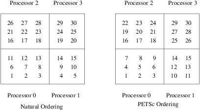
Fig. 3 Natural Ordering and PETSc Ordering for a 2D Distributed Array (Four Processes)

The example SNES Tutorial ex5 illustrates the use of a distributed array in the solution of a nonlinear problem. The analogous Fortran program is SNES Tutorial ex5f; see SNES: Nonlinear Solvers for a discussion of the nonlinear solvers.

Staggered Grids

For regular grids with staggered data (living on elements, faces, edges, and/or vertices), the DMStag object is available. It behaves much like DMDA; see the DMSTAG manual page for more information.

Vectors Related to Unstructured Grids

Index Sets

To facilitate general vector scatters and gathers used, for example, in updating ghost points for problems defined on unstructured grids 1, PETSc employs the concept of an index set, via the IS class. An index set, which is a generalization of a set of integer indices, is used to define scatters, gathers, and similar operations on vectors and matrices.

The following command creates an index set based on a list of integers:

ISCreateGeneral(MPI_Comm comm,PetscInt n,PetscInt *indices,PetscCopyMode mode, IS *is);

When mode is PETSC_COPY_VALUES, this routine copies the n indices passed to it by the integer array indices. Thus, the user should be sure to free the integer array indices when it is no longer needed, perhaps directly after the call to ISCreateGeneral(). The communicator, comm, should consist of all processes that will be using the IS.

Another standard index set is defined by a starting point (first) and a stride (step), and can be created with the command

ISCreateStride(MPI_Comm comm,PetscInt n,PetscInt first,PetscInt step,IS *is);

Index sets can be destroyed with the command

ISDestroy(IS &is);

On rare occasions the user may need to access information directly from an index set. Several commands assist in this process:

ISGetSize(IS is,PetscInt *size);
ISStrideGetInfo(IS is,PetscInt *first,PetscInt *stride);
ISGetIndices(IS is,PetscInt **indices);

The function ISGetIndices() returns a pointer to a list of the indices in the index set. For certain index sets, this may be a temporary array of indices created specifically for a given routine. Thus, once the user finishes using the array of indices, the routine

ISRestoreIndices(IS is, PetscInt **indices);

should be called to ensure that the system can free the space it may have used to generate the list of indices.

A blocked version of the index sets can be created with the command

ISCreateBlock(MPI_Comm comm,PetscInt bs,PetscInt n,PetscInt *indices,PetscCopyMode mode, IS *is);

This version is used for defining operations in which each element of the index set refers to a block of bs vector entries. Related routines analogous to those described above exist as well, including ISBlockGetIndices(), ISBlockGetSize(), ISBlockGetLocalSize(), ISGetBlockSize(). See the man pages for details.

Scatters and Gathers

PETSc vectors have full support for general scatters and gathers. One can select any subset of the components of a vector to insert or add to any subset of the components of another vector. We refer to these operations as generalized scatters, though they are actually a combination of scatters and gathers.

To copy selected components from one vector to another, one uses the following set of commands:

VecScatterCreate(Vec x,IS ix,Vec y,IS iy,VecScatter *ctx);
VecScatterBegin(VecScatter ctx,Vec x,Vec y,INSERT_VALUES,SCATTER_FORWARD);
VecScatterEnd(VecScatter ctx,Vec x,Vec y,INSERT_VALUES,SCATTER_FORWARD);
VecScatterDestroy(VecScatter *ctx);

Here ix denotes the index set of the first vector, while iy indicates the index set of the destination vector. The vectors can be parallel or sequential. The only requirements are that the number of entries in the index set of the first vector, ix, equals the number in the destination index set, iy, and that the vectors be long enough to contain all the indices referred to in the index sets. If both x and y are parallel, their communicator must have the same set of processes, but their process order can be different. The argument INSERT_VALUES specifies that the vector elements will be inserted into the specified locations of the destination vector, overwriting any existing values. To add the components, rather than insert them, the user should select the option ADD_VALUES instead of INSERT_VALUES. One can also use MAX_VALUES or MIN_VALUES to replace destination with the maximal or minimal of its current value and the scattered values.

To perform a conventional gather operation, the user simply makes the destination index set, iy, be a stride index set with a stride of one. Similarly, a conventional scatter can be done with an initial (sending) index set consisting of a stride. The scatter routines are collective operations (i.e. all processes that own a parallel vector must call the scatter routines). When scattering from a parallel vector to sequential vectors, each process has its own sequential vector that receives values from locations as indicated in its own index set. Similarly, in scattering from sequential vectors to a parallel vector, each process has its own sequential vector that makes contributions to the parallel vector.

Caution: When INSERT_VALUES is used, if two different processes contribute different values to the same component in a parallel vector, either value may end up being inserted. When ADD_VALUES is used, the correct sum is added to the correct location.

In some cases one may wish to “undo” a scatter, that is perform the scatter backwards, switching the roles of the sender and receiver. This is done by using

VecScatterBegin(VecScatter ctx,Vec y,Vec x,INSERT_VALUES,SCATTER_REVERSE);
VecScatterEnd(VecScatter ctx,Vec y,Vec x,INSERT_VALUES,SCATTER_REVERSE);

Note that the roles of the first two arguments to these routines must be swapped whenever the SCATTER_REVERSE option is used.

Once a VecScatter object has been created it may be used with any vectors that have the appropriate parallel data layout. That is, one can call VecScatterBegin() and VecScatterEnd() with different vectors than used in the call to VecScatterCreate() as long as they have the same parallel layout (number of elements on each process are the same). Usually, these “different” vectors would have been obtained via calls to VecDuplicate() from the original vectors used in the call to VecScatterCreate().

There is a PETSc routine that is nearly the opposite of VecSetValues(), that is, VecGetValues(), but it can only get local values from the vector. To get off-process values, the user should create a new vector where the components are to be stored, and then perform the appropriate vector scatter. For example, if one desires to obtain the values of the 100th and 200th entries of a parallel vector, p, one could use a code such as that below. In this example, the values of the 100th and 200th components are placed in the array values. In this example each process now has the 100th and 200th component, but obviously each process could gather any elements it needed, or none by creating an index set with no entries.

Vec         p, x;         /* initial vector, destination vector */
VecScatter  scatter;      /* scatter context */
IS          from, to;     /* index sets that define the scatter */
PetscScalar *values;
PetscInt    idx_from[] = {100,200}, idx_to[] = {0,1};

VecCreateSeq(PETSC_COMM_SELF,2,&x);
ISCreateGeneral(PETSC_COMM_SELF,2,idx_from,PETSC_COPY_VALUES,&from);
ISCreateGeneral(PETSC_COMM_SELF,2,idx_to,PETSC_COPY_VALUES,&to);
VecScatterCreate(p,from,x,to,&scatter);
VecScatterBegin(scatter,p,x,INSERT_VALUES,SCATTER_FORWARD);
VecScatterEnd(scatter,p,x,INSERT_VALUES,SCATTER_FORWARD);
VecGetArray(x,&values);
ISDestroy(&from);
ISDestroy(&to);
VecScatterDestroy(&scatter);

The scatter comprises two stages, in order to allow overlap of communication and computation. The introduction of the VecScatter context allows the communication patterns for the scatter to be computed once and then reused repeatedly. Generally, even setting up the communication for a scatter requires communication; hence, it is best to reuse such information when possible.

Scattering Ghost Values

Generalized scatters provide a very general method for managing the communication of required ghost values for unstructured grid computations. One scatters the global vector into a local “ghosted” work vector, performs the computation on the local work vectors, and then scatters back into the global solution vector. In the simplest case this may be written as

VecScatterBegin(VecScatter scatter,Vec globalin,Vec localin,InsertMode INSERT_VALUES, ScatterMode SCATTER_FORWARD);
VecScatterEnd(VecScatter scatter,Vec globalin,Vec localin,InsertMode INSERT_VALUES,ScatterMode SCATTER_FORWARD);
/* For example, do local calculations from localin to localout */
 ...
VecScatterBegin(VecScatter scatter,Vec localout,Vec globalout,InsertMode ADD_VALUES,ScatterMode SCATTER_REVERSE);
VecScatterEnd(VecScatter scatter,Vec localout,Vec globalout,InsertMode ADD_VALUES,ScatterMode SCATTER_REVERSE);

Vectors with Locations for Ghost Values

There are two minor drawbacks to the basic approach described above:

• the extra memory requirement for the local work vector, localin, which duplicates the memory in globalin, and

• the extra time required to copy the local values from localin to globalin.

An alternative approach is to allocate global vectors with space preallocated for the ghost values; this may be done with either

VecCreateGhost(MPI_Comm comm,PetscInt n,PetscInt N,PetscInt nghost,PetscInt *ghosts,Vec *vv)

or

VecCreateGhostWithArray(MPI_Comm comm,PetscInt n,PetscInt N,PetscInt nghost,PetscInt *ghosts,PetscScalar *array,Vec *vv)

Here n is the number of local vector entries, N is the number of global entries (or NULL) and nghost is the number of ghost entries. The array ghosts is of size nghost and contains the global vector location for each local ghost location. Using VecDuplicate() or VecDuplicateVecs() on a ghosted vector will generate additional ghosted vectors.

In many ways, a ghosted vector behaves just like any other MPI vector created by VecCreateMPI(). The difference is that the ghosted vector has an additional “local” representation that allows one to access the ghost locations. This is done through the call to

VecGhostGetLocalForm(Vec g,Vec *l);

The vector l is a sequential representation of the parallel vector g that shares the same array space (and hence numerical values); but allows one to access the “ghost” values past “the end of the” array. Note that one access the entries in l using the local numbering of elements and ghosts, while they are accessed in g using the global numbering.

A common usage of a ghosted vector is given by

VecGhostUpdateBegin(Vec globalin,InsertMode INSERT_VALUES, ScatterMode SCATTER_FORWARD);
VecGhostUpdateEnd(Vec globalin,InsertMode INSERT_VALUES, ScatterMode SCATTER_FORWARD);
VecGhostGetLocalForm(Vec globalin,Vec *localin);
VecGhostGetLocalForm(Vec globalout,Vec *localout);
...  Do local calculations from localin to localout ...
VecGhostRestoreLocalForm(Vec globalin,Vec *localin);
VecGhostRestoreLocalForm(Vec globalout,Vec *localout);
VecGhostUpdateBegin(Vec globalout,InsertMode ADD_VALUES, ScatterMode SCATTER_REVERSE);
VecGhostUpdateEnd(Vec globalout,InsertMode ADD_VALUES, ScatterMode SCATTER_REVERSE);

The routines VecGhostUpdateBegin() and VecGhostUpdateEnd() are equivalent to the routines VecScatterBegin() and VecScatterEnd() above except that since they are scattering into the ghost locations, they do not need to copy the local vector values, which are already in place. In addition, the user does not have to allocate the local work vector, since the ghosted vector already has allocated slots to contain the ghost values.

The input arguments INSERT_VALUES and SCATTER_FORWARD cause the ghost values to be correctly updated from the appropriate process. The arguments ADD_VALUES and SCATTER_REVERSE update the “local” portions of the vector from all the other processes’ ghost values. This would be appropriate, for example, when performing a finite element assembly of a load vector. One can also use MAX_VALUES or MIN_VALUES with SCATTER_REVERSE.

Partitioning discusses the important topic of partitioning an unstructured grid.

1

Also see DMPlex (DMPlex: Unstructured Grids in PETSc), an abstraction for working with unstructured grids.